AMA model structure

Accuracy Maximization Analysis (AMA) is a method to learn the filters that maximize the performance of a probabilistic decoder for a given task.

The goal of this tutorial is to introduce the structure of the AMA model, together with some of the main methods of the amatorch package, which implements AMA in PyTorch.

Different variants of AMA are possible. Here we will present the simplest variant, AMA-Gauss. Other variants are included in amatorch, and the user can also implement custom AMA models. See (fill other tutorials).

Disparity dataset

Disparity

Disparity is the difference in the position of a feature in a pair of binocular (i.e. stereo) images, like the two eyes of a human. Estimating the disparity in an image is a key step in stereo depth perception.

We introduce AMA using a naturalistic disparity dataset that is included in amatorch. The dataset has shape (9500, 2, 26) consisting of 9500 samples, with 2 channels and 26 pixels for each sample, and 19 classes (with 500 samples each) that represent disparity levels in arcmin.

Let’s load the dataset and see the shapes of the tensors:

import matplotlib.pyplot as plt
import numpy as np
import torch
from amatorch.datasets import disparity_data

# Load data and filters
data = disparity_data()
stimuli = data["stimuli"]
labels = data["labels"]
class_values = data["values"]

print(f"Stimuli shape: {list(stimuli.shape)}")
print(f"Labels shape: {list(labels.shape)}")
print(f"Class values: {class_values.numpy()}")

Stimuli shape: [9500, 2, 26]
Labels shape: [9500]
Class values: [-16.875 -15.    -13.125 -11.25   -9.375  -7.5    -5.625  -3.75   -1.875
   0.      1.875   3.75    5.625   7.5     9.375  11.25   13.125  15.
  16.875]

The tensors in the dataset are:

• stimuli: The binocular images, with shape (n_samples, n_channels, n_pixels). For this dataset, n_samples=9500, n_channels=2 (left and right images), and n_pixels=26. amatorch assumes that the input has a channel dimension, so even if there is only one channel, the input should have shape (n_samples, 1, n_pixels).

• labels: The class index for each input, with shape (n_samples).

• class_values: The disparity value of each class in arcmin, with shape (19). The disparity values range from -16.875 to 16.875 arcmin.

Let’s visualize some of the images and their disparities:

plot_inds = torch.tensor([5, 7, 9, 11, 13]) * 501 # Stimuli to plot
fig, ax = plt.subplots(1, len(plot_inds), figsize=(10, 2.5))

for i, ind in enumerate(plot_inds):

    stim_disparity = class_values[labels[ind]]

    ax[i].set_title(f"{stim_disparity} arcmin")
    ax[i].plot(stimuli[ind,0], label="Left image")
    ax[i].plot(stimuli[ind,1], label="Right image")

    ax[i].set_ylim([-0.6, 0.6])
    if i == 0:
        ax[i].set_ylabel("Contrast")
    else:
        ax[i].set_yticklabels([])
    ax[i].set_xlabel("Pixel")

plt.tight_layout()

plt.subplots_adjust(right=0.85)
handles, legend_labels = ax[0].get_legend_handles_labels()
fig.legend(handles, legend_labels, loc='center right',
    bbox_to_anchor=(1.0, 0.5), ncol=1)

plt.show()

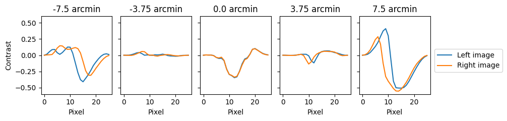
We see that different disparity levels have different shifts between the left and right images. The task is to estimate the disparity level given the binocular image.

Disparity dataset details

Note that the plotted stimuli fade to 0 at the edges, which is a product of a cosine windowing applied to each image. Also note that there are negative and positive pixel values. This is because the image is converted to contrast by subtracting and then dividing by the mean intensity. These two image manipulations are already incorporated in the dataset available in amatorch.

AMA overview

Mathematical notation

Let’s define the following mathematical notation:

• \(s \in \mathbb{R}^d\): The input stimulus, where \(d\) is the number of dimensions.

• \(s^* \in \mathbb{R}^d\): The preprocessed stimulus.

• \(f \in \mathbb{R}^{k \times d}\): The filter matrix where each of the \(k\) rows is a filter.

• \(R \in \mathbb{R}^k\): The response of the filters to \(s*\)

• \(X\): The latent variable, or class, that we want to estimate. In the disparity estimation case, \(X \in \{X_1, ..., X_p\}\) where \(X_j \in \mathbb{R}\) is the disparity value of class \(j\), and \(p\) is the number of classes.

The AMA model consists of three steps:

• Preprocessing

• Encoding

• Probabilistic decoding

The preprocessing step is arbitrary and problem-specific. The default preprocessing in amatorch is to divide each channel of an input by its norm plus a constant:

\[s^* = \frac{s}{\sqrt{s + c_{50}^2}}\]

This is a preprocessing used in previous AMA applications inspired in neural divisive normalization. However, preprocessing can be customized or omitted.

The encoding step obtains a set of filter responses. AMA-Gauss defaults to using linear filtering:

\[R = f s^*\]

Non-linear encodings (such as filter-dependent response normalization) can also be used. The filters \(f\) are the learnable model parameters.

The probabilistic decoding step obtains the posterior distribution over the latent variable given the observed feature responses, \(P(X=X_i|R)\). This uses the class-conditional response distributions \(P(R|X=X_i)\) together with the class priors \(P(X=X_i)\) via Bayes’ rule:

\[ P(X_i|R) = \frac{P(R|X_i)P(X_i)}{P(R)} = \frac{P(R|X_i)P(X_i)}{\sum_{j=1}^p P(R|X_j)P(X_j)} \]

We next describe some of the details of the amatorch implementation of encoding and decoding.

Encoding

Let’s initialize the AMA-Gauss model with pre-trained disparity filters:

from amatorch.datasets import disparity_filters
from amatorch.models import AMAGauss

pretrained_filters = disparity_filters()
torch.set_grad_enabled(False) # We don't need gradients for inference

ama = AMAGauss(
    stimuli=stimuli,
    labels=labels,
    filters=pretrained_filters,
    c50=1.0
)

Note that we need to provide the training inputs and labels at initialization, which will be explained below. We also provide a c50 value that controls the stimulus preprocessing (see above).

Let’s visualize the filters using amatorch.plot:

import amatorch.plot
fig = amatorch.plot.plot_filters(ama, n_cols=4)
fig.set_size_inches(7, 3.5)
plt.tight_layout()
plt.show()

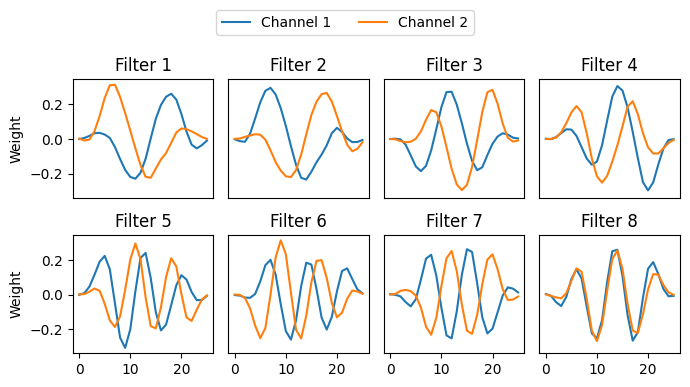
The filters are in the attribute ama.filters and have shape (n_filters, n_channels, n_pixels). They are also an nn.Parameter, so they are learnable.

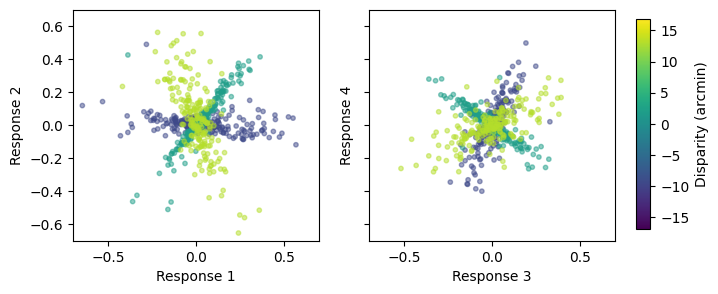
Lets get the filter responses using the method ama.get_responses() and plot the responses for two pairs of filters using the function amatorch.plot.scatter_responses():

responses = ama.get_responses(stimuli)

fig, ax = plt.subplots(1, 2, figsize=(7, 3))
filter_pairs = [(0, 1), (2, 3)]
classes_plot = [4, 10, 16]

for i, filter_pair in enumerate(filter_pairs):
    ax[i] = amatorch.plot.scatter_responses(
      responses=responses,
      labels=labels,
      ax=ax[i],
      values=class_values,
      filter_pair=filter_pair,
      n_points=200,
      classes_plot=classes_plot,
    )

    ax[i].set_xlim([-0.7, 0.7])
    ax[i].set_ylim([-0.7, 0.7])
    if i == 1:
        ax[i].set_yticklabels([])

amatorch.plot.draw_color_bar(colormap="viridis", limits=[-16.875, 16.875],
                             fig=fig, title="Disparity (arcmin)")
plt.show()

Decoding

Response statistics

The filter responses \(R\) have some class-specific response distributions \(P(R|X=X_i)\). If we know the distributions \(P(R|X=X_i)\) and the class priors \(P(X=X_i)\) for each class \(X_i\), we can compute the posterior distribution \(P(X|R)\) over the latent variable given the observed responses as given by Bayes’ rule:

\[ P(X_i|R) = \frac{P(R|X_i)P(X_i)}{\sum_{j=1}^p P(R|X_j)P(X_j)} \]

In the AMA-Gauss model, the class-specific response distributions are assumed to be Gaussian:

\[ P(R|X_i) = \mathcal{N}(\mu_i, \Sigma_i) = \frac{1}{(2\pi)^{k/2}|\Sigma_i|^{1/2}} \exp\left(-\frac{1}{2}(R-\mu_i)^T\Sigma_i^{-1}(R-\mu_i)\right) \]

where \(\mu_i\) and \(\Sigma_i\) are the mean and covariance of the responses for class \(X_i\). Thus, if we know the means and covariances of the responses for each class, we can do probabilistic decoding of the latent variable given the observed responses.

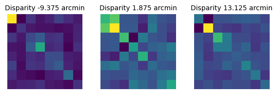
In amatorch models, the parameters defining the response distributions are stored in the attribute ama.response_statistics. For the case of AMAGauss, this attribute is a dictionary with fields 'means' and 'covariances' of shape (n_classes, n_filters) and (n_classes, n_filters, n_filters) respectively. As an example, 3e can visualize the covariance matrices for the classes in the scatter plots above:

# Show the response statistics
response_statistics = ama.response_statistics

fig, ax = plt.subplots(1, 3, figsize=(7, 2))
for i, cind in enumerate(classes_plot):
    ax[i].imshow(response_statistics["covariances"][cind].numpy())
    ax[i].set_title(f"Disparity {class_values[cind]} arcmin", fontsize=10)
    ax[i].axis("off")
plt.show()

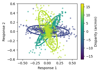
We can also overlay the scatter plots above with the elliptical contours of the class-specific response statistics using amatorch.plot:

fig, ax = plt.subplots(1, figsize=(4, 3))

ax = amatorch.plot.statistics_ellipses(
  means=response_statistics["means"],
  covariances=response_statistics["covariances"],
  filter_pair=(0, 1),
  ax=ax,
  classes_plot=classes_plot,
  values=class_values,
  legend_type="continuous",
  label="Disparity (arcmin)"
)

ax = amatorch.plot.scatter_responses(
  responses=responses,
  labels=labels,
  ax=ax,
  values=class_values,
  filter_pair=(0, 1),
  n_points=500,
  classes_plot=classes_plot,
)

ax.set_xlim([-0.6, 0.6])
ax.set_ylim([-0.6, 0.6])

plt.show()

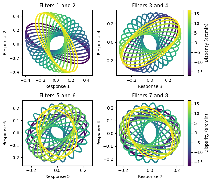
And finally, we can visualize the elliptical contours for all classes and the 4 pairs of filters to get an idea of the statistics for the whole dataset:

filter_pairs = [(0, 1), (2, 3), (4, 5), (6, 7)]
n_cols = 2
width_ratios = [1, 1.2]

fig, ax = plt.subplots(2, 2, figsize=(7, 6), width_ratios=width_ratios)

for i, filter_pair in enumerate(filter_pairs):
    # Calculate row and column indices
    row = i // n_cols
    col = i % n_cols

    if col == 1:
        legend_type = "continuous"
    else:
        legend_type = "none"

    ax[row, col] = amatorch.plot.statistics_ellipses(
      means=response_statistics["means"],
      covariances=response_statistics["covariances"],
      filter_pair=filter_pair,
      ax=ax[row, col],
      values=class_values,
      legend_type=legend_type,
      label="Disparity (arcmin)"
    )

    ax[row, col].set_title(f"Filters {filter_pair[0]+1} and {filter_pair[1]+1}")

plt.tight_layout()
plt.show()

How are the class-specific statistics \(\mu_i\) and \(\Sigma_i\) obtained? Unlike the filters, which are learned by gradient descent, the conditional response distributions are not learnable parameters. Instead, they are computed from the training set and the filters. Thus, they need to be recomputed after every change in the filters (e.g. after every training iteration), which is done by amatorch automatically.

This property of ama explains why when we initialize the AMAGauss model, we need to provide the stimuli and labels, because these are later used to compute the conditional response distributions. The stimulus properties needed to compute the response statistics are stored in the attribute ama.stimulus_statistics, and these are dependent on the AMA model variant.

Gradients of the response statistics

Importantly, the decoding of a given stimulus depends on both the filter responses to that stimulus and the filter response statistics to the training dataset. Because these both depend on the filters, it is important to take into account the gradient of the response statistics with respect to the filters. Thus, the attribute ama.response_statistics determining the conditional response distributions keeps track of gradients.

Response decoding

To decode the latent variable we start by computing the probability of the responses given each class, \(P(R|X_i)\). This probability as a function of \(X_i\) is the likelihood of the latent variable. Let’s visualize this for a single stimulus, by overlaying the response to the single stimulus with the class-specific response statistics. We also plot the likelihood of the disparities, obtained with the method ama.responses_2_log_likelihoods():

# Plot a single stimulus response and the resulting posterior
fig, ax = plt.subplots(1, 3, figsize=(10, 3.5), width_ratios=[1.2, 2, 1.2])
i = 1793 # Stimulus to plot

# Plot the stimulus
ax[0].plot(stimuli[i,0].numpy(), label="Left image")
ax[0].plot(stimuli[i,1].numpy(), label="Right image")
ax[0].legend()
ax[0].set_title(f"Stimulus with disparity {class_values[labels[i]]} arcmin")

# Plot the statistics and stimulus response
ax[1] = amatorch.plot.statistics_ellipses(
  means=response_statistics["means"],
  covariances=response_statistics["covariances"],
  ax=ax[1],
  values=class_values,
  legend_type="continuous",
  label="Disparity (arcmin)"
)

ax[1].scatter(
  responses[i, 0],
  responses[i, 1],
  color="red",
  label="Response",
  s=100
)
ax[1].set_title("Response and statistics")
ax[1].legend()

# Plot the stimulus likelihood
stim_likelihood = ama.responses_2_log_likelihoods(responses[i])
ax[2].plot(class_values, torch.exp(stim_likelihood))
ax[2].set_xlabel("Disparity")
ax[2].set_ylabel("Likelihood")
ax[2].set_title("Stimulus likelihood")

plt.tight_layout()
plt.show()

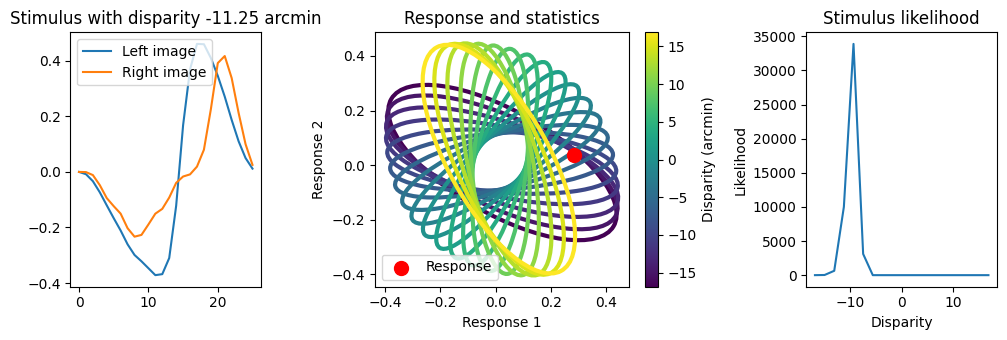
Note that the response to the stimulus is much closer to the ellipses for negative disparities (purple) than for positive disparities (the true disparity is negative). This is reflected in the likelihood plot, with the most likely disparities being negative.

Inference methods

The amatorch models have different methods to compute the intermediate steps encoding-decoding, which consist of the responses, likelihoods, posteriors and estimates. There are methods get_responses(), get_log_likelihoods(), get_posteriors() and get_estimates(), all which take the stimuli as input. There are also methods that perform each of these steps: responses_2_log_likelihoods(), log_likelihoods_2_posteriors() and posteriors_2_estimates(), each taking as input the output of the previous step. By default, the estimate returned by AMA is the index of the maximum posterior category.

Let’s now plot the posterior distribution of the latent variable for this stimulus, and show the maximum posterior estimate:

# Plot the posterior of the model for this stimulus
posteriors = ama.get_posteriors(stimuli)
max_posterior = class_values[ama.get_estimates(stimuli[i])]

fig, ax = plt.subplots(1, figsize=(4, 2))
ax.plot(class_values, posteriors[i])
ax.set_xlabel("Disparity")
ax.set_ylabel("Posterior")
ax.axvline(max_posterior, color="black", linestyle="--", label="Estimate")
ax.axvline(class_values[labels[i]], color="red", linestyle="--", label="True disparity")
ax.legend()
plt.show()

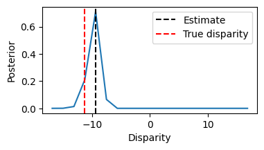
We see that the posteriors looks like the likelihood. This is because the default priors are uniform, and we did not set the priors when initializing the model. Priors \(P(X=X_i)\) are stored in the attribute ama.priors, let’s print them to verify that they are flat:

print(ama.priors)

tensor([0.0526, 0.0526, 0.0526, 0.0526, 0.0526, 0.0526, 0.0526, 0.0526, 0.0526,
        0.0526, 0.0526, 0.0526, 0.0526, 0.0526, 0.0526, 0.0526, 0.0526, 0.0526,
        0.0526])

Finally, we saw that for our example stimulus, the posterior didn’t peak at the true disparity. Let’s see how the model performs over all the stimuli for this class, by plotting all individual posteriors, the mean posterior, and the maximum of the mean posterior:

class_ind = 3

mean_posteriors = torch.mean(posteriors[labels == class_ind], axis=0)
max_posterior_ind = torch.argmax(mean_posteriors)
max_posterior_value = class_values[max_posterior_ind]

fig, ax = plt.subplots(1, figsize=(4, 3))

ax.plot(class_values, posteriors[labels == class_ind].T, color="gray", alpha=0.2)
ax.plot([], [], color="gray", label="Individual posteriors", alpha=0.1) # For legend
ax.plot(class_values, mean_posteriors, color="black", label="Mean posterior")
ax.set_xlabel("Disparity")
ax.set_ylabel("Posterior")
ax.axvline(max_posterior_value, color="black", linestyle="--", label="Max mean posterior")
ax.axvline(class_values[labels[i]], color="red", linestyle="--", label="True disparity")
ax.legend()
plt.show()

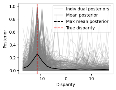
We see that the average posterior peaks at the true disparity, but that there is considerable variability in the posterior across stimuli.

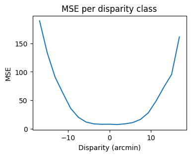
Finally, let’s evaluate the performance of the model. First, lets compute the mean squared error (MSE) between the true disparities and the maximum posterior estimates, both for the whole dataset and for each class:

estimates_inds = ama.posteriors_2_estimates(posteriors)
estimates_values = class_values[estimates_inds]

total_mse = torch.mean((class_values[labels] - estimates_values)**2)
class_mse = torch.zeros(len(class_values))
for i in range(len(class_values)):
    class_mse[i] = torch.mean((class_values[i] - estimates_values[labels == i])**2)

print(f"Total MSE: {total_mse}")

fig, ax = plt.subplots(1, figsize=(4, 3))
plt.plot(class_values, class_mse)
plt.xlabel("Disparity (arcmin)")
plt.ylabel("MSE")
plt.title("MSE per disparity class")
plt.show()

Total MSE: 53.56591033935547

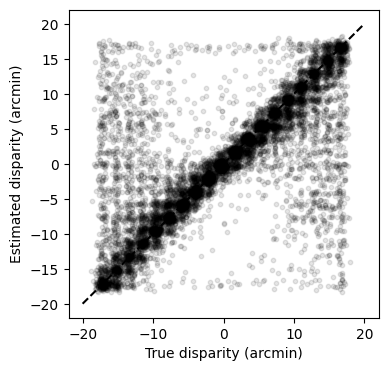
Second, lets scatter the estimated vs true disparities (we add some jitter to the points to avoid overplotting):

fig, ax = plt.subplots(1, figsize=(4, 4))
jitter_x = 0.5 * torch.randn(len(labels)) - 0.25
jitter_y = 0.5 * torch.randn(len(labels)) - 0.25

ax.scatter(class_values[labels] + jitter_x, estimates_values + jitter_y, alpha=0.1,
           s=10, color="black")
ax.plot([-20, 20], [-20, 20], color="black", linestyle="--")
ax.set_xlabel("True disparity (arcmin)")
ax.set_ylabel("Estimated disparity (arcmin)")
plt.show()

Summary

In this tutorial we introduced the structure of AMA models, showing how to interact with amatorch to initialize a model, encode the stimuli, and perform probabilistic decoding. We showed how to use amatorch.plot to visualize the model parameters and attributes (filters and response statistics), as well as the responses, likelihoods, posteriors and estimates for a single stimulus and for the whole dataset.

In coming up tutorials we will show how to train AMA models, other variants of AMA, and how to implement custom AMA models.